Stochastic Differential Equations

An autonomous SDE can be written as

\[X(t) = X(0) + \int_{0}^{t}f(X(s))ds + \int_{0}^{t}g(X(s))dW(s)\]

or formally

\[dX(t) = f(X(t))dt + g(X(t))dW(t)\]

In this section, we will showcase how to use our package to solve SDEs numerically.

The Euler-Maruyama Method

The Eular-Maruyama method is fairly intuitive. It approximates the integrals via their left-most points.

\[\begin{split}\begin{align*} X_j &= X_{j-1} + \int_{t_{j-1}}^{t_j}f(X(s))ds + \int_{t_{j-1}}^{t_j}g(X(s))dW(s)\\ &\approx X_{j-1} + f(X(t_{j-1}))\int_{t_{j-1}}^{t_j}ds + g(X(t_{j-1}))\int_{t_{j-1}}^{t_j}dW(s)\\ \end{align*}\end{split}\]

In “differential” form, we have

\[X_j = X_{j-1} + f(X_{j-1})\Delta t + g(X_{j-1})(W(\tau_j) - W(\tau_{j-1}))\]

To demonstrate, we use the linear SDE:

\[dX(t) = \lambda X(t)dt + \mu X(t)dW(t)\]

As a matter of fact, we have the analytical solution to this SDE:

\[X(t) = X(0)\exp((\lambda - \dfrac{1}{2}\mu^2)t + \mu W(t))\]

We will take \(\lambda=2, ~ \mu=1\) and \(X_0=1\)

from sde.sde_class import sde_class
import numpy as np
from matplotlib import pyplot as plt
# Generate BM
sde = sde_class(T=1, N=10000, M=1000)
# Define drift and diffusion
def mu_fun(x):
    return 2 * x
def sigma_fun(x):
    return x
# EM
X_dict = {}
for R in [1,2,128,256]:
    X = sde.euler_maruyama(mu_fun=mu_fun,
                            sigma_fun=sigma_fun,
                            x0=1,
                            R=R)
    X_dict[R] = X
# Visualize the first path
plt.style.use('ggplot')
for R in X_dict:
    plt.plot(sde.time[::R], X_dict[R][0,:],
            label='EM with R='+str(R),
            linewidth=1)
plt.plot(sde.time, np.exp((2-0.5)*sde.time + sde.W[0,:]),
        label="Truth",
        linewidth=1)
plt.legend()
plt.xlabel("Time")
plt.ylabel("X(t)")
plt.tight_layout()

You should get something similar to this:

Milstein’s Higher Order Method

As we shall see in Convergence and Stability, the EM method, albeit being intuitive, has a suboptimal strong order of convergence. The Milstein’s method improves upon this. However, this does come with additional cost of computing the derivatives of the diffusion function.

Instead of using the left-most points, we exploit Ito’s formula.

\[\begin{split}\begin{align*} d(f(X_t)) &= (f'f + \dfrac{1}{2}f'' g^2)dt + (f'g)dW_t\\ d(g(X_t)) &= (g'f + \dfrac{1}{2}g'' g^2)dt + (g'g)dW_t\\ X_{j} &= X_{j-1} + \int_{t_{j-1}}^{t_j}(f_{j-1} + \int_{t}^{s}(f'f + \dfrac{1}{2}f'' g^2)du + \int_{t}^{s}(f'g)dW_u)ds\\ &+ \int_{t_{j-1}}^{t_j}(g_{j-1} + \int_{t}^{s}(g'f + \dfrac{1}{2}g'' g^2)du + \int_{t}^{s}(g'g)dW_u)dW_s \end{align*}\end{split}\]

Dropping terms higher than \(O(dt)\), we have

\[\begin{split}X_{j} &= X_{j-1} + \int_{t_{j-1}}^{t_j}f_{j-1} ds\\ &+ \int_{t_{j-1}}^{t_j}(g_{j-1} + \int_{t}^{s}(g'g)dW_u)dW_s\\ &= X_{j-1} + f_{j-1}\Delta t\\ &+ g_{j-1}(W_{j} - W_{j-1}) + \int_{t_{j-1}}^{t_j}(\int_{t}^{s}(g'g)dW_u)dW_s\end{split}\]

We then apply the Eular-Maruyama on the last term,

\[\begin{split}\begin{align*} \int_{t_{j-1}}^{t_j}(\int_{t}^{s}(g'g)dW_u)dW_s &\approx (g_{j-1}'g_{j-1})\int_{t_{j-1}}^{t_j}(\int_{t}^{s}dW_u)dW_s\\ &= (g_{j-1}'g_{j-1})\int_{t_{j-1}}^{t_j}(W_s - W_t)dW_s\\ &= (g_{j-1}'g_{j-1})(\int_{t_{j-1}}^{t_j}W_sdW_s - W_{j-1}(W_{j}-W_{j-1}))\\ &= (g_{j-1}'g_{j-1})(\dfrac{1}{2}W_j^2 - \dfrac{1}{2}W_{j-1}^2 - \dfrac{1}{2}\Delta t - W_{j-1}(W_{j}-W_{j-1}))\\ &= \dfrac{1}{2}(g_{j-1}'g_{j-1})((W_{j}-W_{j-1})^2 - \Delta t) \end{align*}\end{split}\]

Therefore, it takes the form of

\[\begin{split}X_j = X_{j-1} + \Delta tf(X_{j-1}) + g(X_{j-1})(W(\tau_j) - W(\tau_{j-1})) + \\ \dfrac{1}{2}g(X_{j-1})g'(X_{j-1})((W(\tau_j) - W(\tau_{j-1}))^2 - \Delta t)\end{split}\]

Continuing with the previous example, we can carry out the Milstein’s method as follows:

# Define derivative function
def d_sigma_fun(x):
    return 1
# Compute Milstein method
m_X_dict = {}
for R in [1,2,128,256]:
    X = sde.milstein(mu_fun=mu_fun,
                    sigma_fun=sigma_fun,
                    d_sigma_fun=d_sigma_fun,
                    x0=1,
                    R=R)
    m_X_dict[R] = X
# Visualize the first path
plt.style.use('ggplot')
for R in m_X_dict:
    plt.plot(sde.time[::R], X_dict[R][0,:],
            label='Milstein with R='+str(R),
            linewidth=1)
plt.plot(sde.time, np.exp((2-0.5)*sde.time + sde.W[0,:]),
        label="Truth",
        linewidth=1)
plt.legend()
plt.xlabel("Time")
plt.ylabel("X(t)")
plt.tight_layout()

You should get something similar to this:

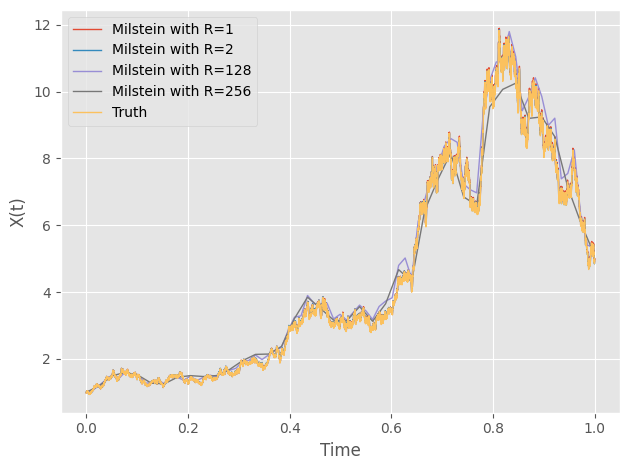
Although the two methods look really similar to each other, we can compare the errors at the end point among the time steps

# Compute errors
error_df = []
for R in X_dict:
    for path in range(1000):
        error_df.append(["EM", R, X_dict[R][path,-1] - np.exp((2-0.5)*1 + sde.W[path,-1])])

for R in m_X_dict:
    for path in range(1000):
        error_df.append(["Milstein", R, m_X_dict[R][path,-1] - np.exp((2-0.5)*1 + sde.W[path,-1])])

error_df = pd.DataFrame(error_df, columns=["Method", "R", "Error"])
# Side-by-side boxplot
sns.boxplot(data=error_df,
            hue='Method',
            x="R",
            y="Error",
            palette="bright")
plt.ylim([-1,1])
plt.show()

As we can see, as the step grows larger, the errors grow larger, too. For exploration on convergence, check out Convergence and Stability

Stochastic Chain Rule

Another interesting aspect of stochastic calculus is its chain rule (a.k.a Ito’s formula). We can illustrate its validity using simulation.

This time we consider the SDE

\[dX(t) = (\alpha - X(t))dt + \beta \sqrt{X(t)}dW(t)\]

with \(\alpha=2, ~ \beta=1, ~ X_0=1\). We consider the function \(V(X)=\sqrt{X}\). Then, by Ito’s formula we know that

\[dV(t) = (\dfrac{4\alpha - \beta^2}{8V(t)}-\dfrac{1}{2}V(t))dt + \dfrac{1}{2}\beta dW(t)\]

We will use EM method to compute these two SDEs and compare their results.

# Generate a BM
sde = sde_class(T=1, N=1000, M=1)
# Define mu and sigma
def x_mu_fun(x):
    return 2-x
def x_sigma_fun(x):
    return 1*np.sqrt(x)
def v_mu_fun(v):
    return (4*2 - 1)/(8*v) - 0.5 * v
def v_sigma_fun(v):
    return 0.5 * 1
# EM
X = sde.euler_maruyama(mu_fun=x_mu_fun,
                    sigma_fun=x_sigma_fun,
                    x0=1)
V = sde.euler_maruyama(mu_fun=v_mu_fun,
                    sigma_fun=v_sigma_fun,
                    x0=1)
# Compare results
plt.style.use('ggplot')
plt.plot(sde.time, V[0,:],
        label="Chain Rule",
        c='magenta')
plt.plot(sde.time, np.sqrt(X[0,:]),
        label="Direct",
        c="cyan")
plt.xlabel("Time")
plt.ylabel("V(t)")
plt.legend()
plt.tight_layout()
plt.show()

We see that there is good agreement between these two methods.