Stochastic Integrals
Ito Integrals
One of the most fundamental tools in SDE is Ito integral. The basic idea is to mimic the Riemann sum but only with the left-most point. (The process is thus non-anticipating)
In its discrete form, suppose we have a function \(h(t)\), then its “Ito” sum is
By using our package, you can easily compute the approximate Ito integral. To demonstrate, suppose \(h(t)=W(t)\). This is actually one of the rare cases where we can find the analytical solution
Tip
Wondering how it’s done? Just use the definition.
from sde.sde_class import sde_class
import numpy as np
from matplotlib import pyplot as plt
# Initialize sde_class object
sde = sde_class(T=1, N=1000, M=1000)
# Define integrand
def h(t, w):
return w
# Ito integral
results = sde.integrate(fun=h,
integral_type="Ito")
# Visualize the results
plt.style.use('ggplot')
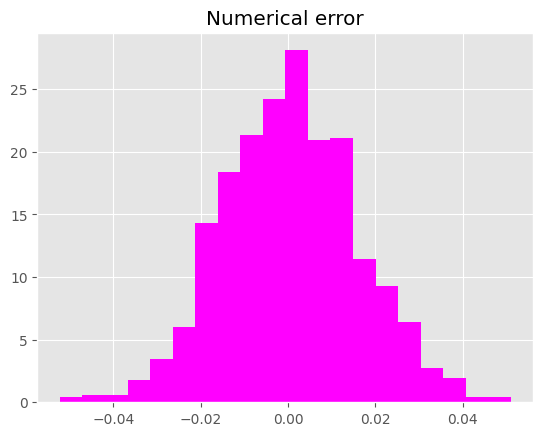
plt.hist(results - 0.5*sde.W[:,-1]**2 + 0.5,
bins=20, density=True, color="magenta")
plt.title("Numerical error")
plt.show()
You should get something similar to this:
Stratonovich Integrals
Ito integral approximates using the left-most point. In practice, there is nothing stopping you from using any other point in between. Stratonovich integral uses the middle point.
Again, we will use \(h(t)=W(t)\) to demonstrate. The analytical solution is given by
Tip
Wondering how it’s done? Think about how you would impute the middle point of Brownian Motions positions.
Let \(W_1 = W(t_j), W_2 = W(\lambda t_{j+1} + (1-\lambda)t_j), W_3 = W(t_{j+1}), ~ \Delta = t_{j+1}-t_j\)
# Stratonovich integral
results = sde.integrate(fun=h,
integral_type="Stratonovich")
# Visualize the results
plt.style.use('ggplot')
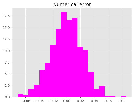
plt.hist(results - 0.5*sde.W[:,-1]**2,
bins=20, density=True, color="magenta")
plt.title("Numerical error")
plt.show()
You should get something similar to this: