Convergence and Stability
So I see you are of the paranoid type and get suspicious about numerical methods. That’s what this section is for. We demonstrate by using our package various aspects of convergence of the numerical methods we included in the package.
Note
The simulation in the paper might take a looooong time to run.
The SDE we will use is the same as the one we investigated in Stochastic Differential Equations
Strong Convergence
A method is said to have strong order of convergence equal to \(\gamma\) if
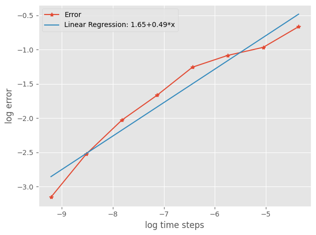
The Eular-Maruyama (EM) method can be shown to have strong order of convergence \(\gamma=\dfrac{1}{2}\). To validate this, we can simulate multiple Brownian Motions, compute the SDE using the EM method, and compare the absolute errors with the ground truth.
# Generate BMs
sde = sde_class(T=1, N=10000, M=1000)
# Define mu and sigma functions
def mu_fun(x):
    return 2 * x
def sigma_fun(x):
    return x
# Define time steps
R_seq = np.array([1,2,4,8,16,32,64,128])
X_dict = {}
for R in R_seq:
    X = sde.euler_maruyama(mu_fun=mu_fun,
                        sigma_fun=sigma_fun,
                        x0=1,
                        R=R)
    X_dict[R] = X
# Compute errors
error_df = []
for R in X_dict:
    rows = [[err, R] for err in np.abs(X_dict[R][:,-1] - \
            np.exp((2-0.5) + sde.W[:,-1]))]
    error_df += rows
error_df = pd.DataFrame(error_df, columns=["Error", "R"])
# Compute group mean and lr
log_err = np.log(error_df.groupby(['R'])['Error'].mean().values)
m, b = np.polyfit(np.log(sde.dt * R_seq), log_err,1)
# Visualize the results
plt.style.use('ggplot')
plt.plot(np.log(sde.dt * R_seq),
        log_err, marker="*",
        label="Error")
plt.plot(np.log(sde.dt * R_seq),
        m*np.log(sde.dt * R_seq)+b,
        label="Linear Regression: "+
        str(np.round(b,2)) +
        "+" + str(np.round(m,2))+"*x")
plt.xlabel("log time steps")
plt.ylabel("log error")
plt.tight_layout()
plt.legend()
plt.show()
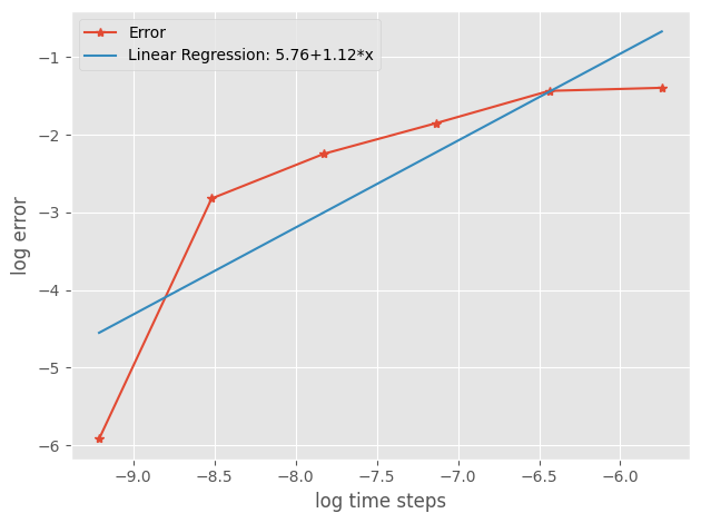
We can also validate the strong order of convergence of the Milstein’s method is 1.
# Generate BMs
sde = sde_class(T=1, N=10000, M=1000)
# Define mu and sigma functions
def mu_fun(x):
    return 2 * x
def sigma_fun(x):
    return x
def d_sigma_fun(x):
    return 1
# Milstein
R_seq = np.array([1,2,4,8,16,32])
X_dict = {}
for R in R_seq:
    X = sde.milstein(mu_fun=mu_fun,
                    sigma_fun=sigma_fun,
                    d_sigma_fun=d_sigma_fun,
                    x0=1,
                    R=R)
    X_dict[R] = X
# Compute error
error_df = []
for R in X_dict:
    rows = [[err, R] for err in np.abs(X_dict[R][:,-1] - \
            np.exp((2-0.5) + sde.W[:,-1]))]
    error_df += rows
error_df = pd.DataFrame(error_df, columns=["Error", "R"])
# Visualize
log_err = np.log(error_df.groupby(['R'])['Error'].mean().values)
m,b = np.polyfit(np.log(sde.dt * R_seq), log_err,1)
plt.style.use('ggplot')
plt.plot(np.log(sde.dt * R_seq),
        log_err, marker="*",
        label="Error")
plt.plot(np.log(sde.dt * R_seq),
        m*np.log(sde.dt * R_seq)+b,
        label="Linear Regression: "+
        str(np.round(b,2)) +
        "+" + str(np.round(m,2))+"*x")
plt.xlabel("log time steps")
plt.ylabel("log error")
plt.tight_layout()
plt.legend()
plt.show()
Weak Convergence
A method is said to have weak order of convergence equal to \(\gamma\) if
The Eular-Maruyama (EM) method can be shown to have weak order of convergence \(\gamma=1\). To validate this, we can simulate multiple Brownian Motions, compute the SDE using the EM method, and compare the absolute errors with the ground truth.
def mu_fun(x):
    return 2 * x
def sigma_fun(x):
    return 0.1*x
R_seq = np.array([1,2,4,8,16,32,64,128])
EX = np.zeros(len(R_seq))
for i, R in enumerate(R_seq):
    sde = sde_class(T=1, N=1000, M=5000)
    X = sde.euler_maruyama(mu_fun=mu_fun,
                        sigma_fun=sigma_fun,
                        x0=1,
                        R=R)
    EX[i] = np.mean(X[:,-1])
# Compute error and visulalize
m, b = np.polyfit(np.log(sde.dt * R_seq),
                np.log(np.abs(EX-np.exp(2))),1)
plt.style.use('ggplot')
plt.plot(np.log(sde.dt * R_seq),
        np.log(np.abs(EX-np.exp(2))), marker="*",
        label="Error")
plt.plot(np.log(sde.dt * R_seq),
        m*np.log(sde.dt * R_seq)+b,
        label="Linear Regression: "+
        str(np.round(b,2)) +
        "+" + str(np.round(m,2))+"*x")
plt.xlabel("log time steps")
plt.ylabel("log error")
plt.tight_layout()
plt.legend()
plt.show()

Linear Stability
Stability mainly concerns with the ability of a method to reproduce a certain qualitative feature of an SDE.
In this section, we will again use
And the feature we are interested in is \(\underset{t\to\infty}{\lim}X(t)=0\) (Of course in some “probability” sense).
There are metrics we will use
As we know the analytic solution, we know the conditions we need to impose on \(\lambda, \mu\).
Given the region of \(\lambda, \mu\), we are interested in finding out the time steps of the Eular-Maruyama that can reproduce these features.
Based on the EM method, we have for mean-square stability
This yields \((1+\lambda dt)^2 + \mu^2 dt<1\)
For asymptotic stability,
We than normalize both sides with mean \(m\) and variance \(s^2\),
Now if \(E\log|(1+\lambda dt + \mu dWt) < 0\), we have
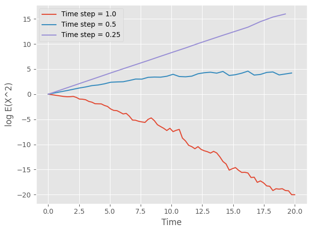
Mean-Square Stability
#Generate BMs
sde = sde_class(T=20, N=80, M=50000)
# EM
def mu_fun(x):
    return -3 * x
def sigma_fun(x):
    return np.sqrt(3)*x
R_seq = np.array([1,2,4])
X_dict = {}
for R in R_seq:
    X = sde.euler_maruyama(mu_fun=mu_fun,
                        sigma_fun=sigma_fun,
                        x0=1,
                        R=R)
    X_dict[R] = X
# Visualize mean-square
for R in X_dict:
    plt.plot(sde.time[::R],
            np.log10(np.mean(X_dict[R]**2, axis=0)),
            label="Time step = "+str(1/R))
plt.xlabel("Time")
plt.ylabel("log E(X^2)")
plt.tight_layout()
plt.legend()
plt.show()
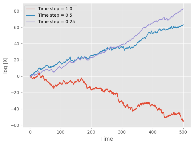
Asymptotic
# Generate BMs and carry out EM
sde = sde_class(T=500, N=2000, M=1)
def mu_fun(x):
    return 0.5 * x
def sigma_fun(x):
    return np.sqrt(6)*x
R_seq = np.array([1,2,4])
X_dict = {}
for R in R_seq:
    X = sde.euler_maruyama(mu_fun=mu_fun,
                        sigma_fun=sigma_fun,
                        x0=1,
                        R=R)
    X_dict[R] = X

# Visualize asymptotic
for R in X_dict:
    plt.plot(sde.time[::R],
            np.log10(np.abs(X_dict[R][0,:])),
            label="Time step = "+str(1/R))
plt.xlabel("Time")
plt.ylabel("log |X|")
plt.tight_layout()
plt.legend()
plt.show()